
Fig. 1. A pure two-tone signal as seen on an oscilloscope.
The third order intercept point. (IP3)BackgroundThis is the definition: The third order intercept point (IP3) is the point at which the the extrapolated third order intermodulation level (IM3) is equal to the signal levels in the output of a two-tone test when the extrapolation is made from a point below which the third order intermodulation follows the third order law. IP3 may be given as the input level or as the output level for that point and which one has to be specified. One uses the terms input intercept point IIP3 and output intercept point OIP3.The third order law says that the intermodulation product grows with the input amplitude raised to a power of three. The intermodulation will grow by 3 dB for a single dB increase of the input. IP3 is a figure of merit that characterizes a receiver's tolerance to several signals that are present simultaneously outside the desired passband. IP3 is a power level, typically given in dBm, and it is closely related to the 1 dB compression point. Both IP3 and the 1 dB compression point are meaningful only when given in relation to the noise floor. Adding a 10 dB attenuator to a receiver will improve both IP3 and the 1 dB compression point by 10 dB, but it will also degrade the system noise figure by 10 dB so the 10 dB attenuator is not improving the dynamic range, it just shifts the power range upwards. The third order intercept point, IP3, although a number that is obtained from an extrapolation, has a real physical meaning and it is well defined. The fact that different standardized procedures give different results may be because not all of these procedures measure IP3 correctly. They may be based on incorrect assumptions or some theoretical mistake. There may also be overtones of the test signals present. This article Receiver Dynamic Range which has appeared in DUBUS and CQ VHF discusses some practical aspects of IM3 measurements. Another thing is that IP3 and the theory behind it is not applicable on all receivers. In such cases the number that comes out of a standardized procedure will not be IP3, it will just be the outcome of a specific procedure. The most obvious case is a DSP radio containing an A/D converter in the signal path. If both test signals reach the A/D converter, IM3 will not have any tendency at all to follow a third order law at low signal levels. More here: IMD in Digital Receivers QEX Nov/Dec 2006, pp 18 - 22. See also Dynamic range observations for the SDR-14 Analog receivers may have side circuits such as noise blankers that contain amplifiers, detectors or other circuits that produce intermodulation at signal levels where the main signal path is very linear. Such intermodulation may leak into the main signal path due to inadequate screening or buffering causing irregular behaviour at low signal levels, thus making IP3 and the associated theory invalid. A perfectly linear amplifier will have no intermodulation at all, but at some point it must saturate. The third order intermodulation associated with abrupt saturation does not follow the third order law, something that can be seen on the plot of the Delta44 below. IP3 is a figure of merit that is useful to characterize the linearity of a receiver for signals well below saturation. IP3 is typically a function of the frequency separation. Stages that are preceeded by filters that remove one (or both) of the test signals will not contribute to IM3 in a two tone test, but as the frequency separation is made narrower, both test tones will pass through more of the filters and cause IM3 further into the receiver, usually with a much lower IP3 than the one associated with the front-end. In some cases IM3 at very low signal levels has been reported to be orders of magnitude stronger than expected. For example the review of TS-450S and TS-690S in QST April 1992 shows IM3 at the noise floor for an input signal of -64 dBm while the third order law gives the expected IM3 level about 60 dB lower. If the phenomenon is real, the reason for the very strong intermodulation at low signal levels is most probably some side-circuit. Something non-linear that receives an amplified signal and produces intermodulation that leaks into the main signal path due to inadequate isolation. I have measured the IM3 produced in a TS-690S at the RS-03 meeting and did not see any trace of low level IM3. The serial number was much later compared to the 1992 ARRL Lab test, Kenwood may have corrected whatever problem that was present in early TS-690S units - or maybe there was a problem with the ARRL measurements. Excessive IM3 at low levels has been reported implicitly in several tests from the ARRL lab as shown in table 1. |
Table 1 Deviations from the third order law as calculated from ARRL equipment reviews by the formula IP3=1.5*IM3DR+MDS |
|
It has to be understood that ARRL Lab has its own definition of IP3: "IP3 is the result of a third order extrapolation of the IM3 response at the S5 level" This procedure surely gives an accurate value for IP3 for all receivers that really follow a third order law, but back in 1992 when the TS-690S was measured, ARRL Lab used another definition of IP3. The TS-690S IM3 value at the noise floor was extrapolated with a slope of 3 leading to a published IP3 value of -33 dBm. With today's procedure, extrapolating from the S5 level, one gets a line that crosses the signal at about +4 dBm from the very same measurement. The difference between the old and the new procedure is 37 dB!! None of the methods is acceptable. A receiver that has a third order response like TS-690S in the ARRL Lab test does not have any IP3 at all. IP3 must not be redefined to be the outcome of a procedure. IP3 is a well defined quantity that has a good theoretical model behind it. Some receivers may contain circuits that make the model incorrect and in such cases one can not use a concept from the model. The TS-450S/TS-690S units measured at the ARRL Lab probably have an IP3 of +5 dBm for the front-end as determined from Fig A in QST April 1992 page 70. A measurement at 100 kHz separation would probably have shown a normal third order response since the two tones would probably not have reached the circuits responsible for the irregular behaviour in case the observation was real and not an artifact. There is an article in QEX Jul/Aug 2002 p. 50, in which Ed Hare, the ARRL Lab Supervisor argues that there is not a true intercept point for a receiver because the IM3 curves do not follow the third order law. This statement is fine, but the three different response curves in this very article are however not good examples. The curves giving "IP3 from MDS" are not drawn correctly. The response curves show the reading of an RMS voltmeter and they are curves showing S+N. The position of the noise floor is known and the correct point to draw the lines from is a point 3 dB below the point where the S+N response is 3 dB above the noise floor. At this point S and N are equal, both S and N are 3 dB below the sum of both of them. The line drawn from the correct place at the MDS level coincides exactly with the line "IP3 from Best Fit in Linear Output Range" in Fig C and the answer to the question at the side of fig. C: "What is the 'real' intercept point of this icom IC-765?" is IP3 = +9.5 dBm. The third line in fig C is not compatible with the definition of IP3. This non-linearity may be caused by loss of gain in which case it would disappear if a third signal were used to keep track of receiver gain variations as shown in fig 11 below. Table 1 and the published result for the TS-450S indicate that IP3 is not a useful figure of merit for some receivers because there is no point below which IM3 follows the third order law. For receivers having large discrepancies, IP3 should not be given at all, one has to specify some signal levels and the corresponding IM3 levels. Best, of course with a diagram as was done for the TS-690S, but for the receivers in table 1, giving IM3 below the signal level for a test signal pair X dB above the noise floor would be a better way to present the results. It is my personal belief that any analog radio that gives much more IM3 at low levels than one would expect from the third order law suffers from an easily correctable design error. Table 1 may be an example of such receivers. I have tried to find a receiver that has high IM3 levels when the measurement is made at the noise floor because I would like to investigate the mechanism. I have not yet found a single one. Measurements at the noise floor are difficult, the phenomenon could be an artifact. I will continue searching for it by bringing instruments to ham meetings. Details of performance measurements are given here. TheoryLet us start by looking at the intermodulation generated in a single building block of a receiver. It could be an amplifier, a mixer, a ferrite core or something else. A single stage that causes intermodulation can be described by a transfer function that is very close to a straight line for voltages well below saturation. If the input is denoted X(t), a voltage that varies with time, the output Y(t+d) can be described with a power-series expansion in amplitudes only:Y(t+d) = k1X(t)+ k2{X(t)}2 + k3{X(t)}3 + …......... (1) where k1, k2, k3 etc. are constant coefficients and d is the time delay between input and output (not important here). Such a description is valid if the input signal is small. At larger signal levels, there will also be a phase shift because semiconductors contain a capacitance that varies with the voltage in a non-linear fashion. Any reasonable analog circuitry will have k1 > k2 > k3 >… so if the signal levels are really low, the transfer function is well described by the first ‘linear’ term only. By making X(t)=A*{ sin(2*PI*f1) + sin(2*PI*f2) } one can easily find what the output signal Y(t+d) becomes in a two-tone test on a unit that is described by the polynomial expansion (1). X(t) is two sine waves of equal amplitude A and with frequencies f1 and f2. Look here for the mathematical details The result for the third order intermodulation amplitudes is: IM3=0.5*k3*A3+ 1.5*k5*A5 + 3*k7A7 + …......... (2) Here k3 is in the order of 0.06 if the amplitude A is expressed in units of the voltage at the 1 dB compression point. When two analog building blocks that both are well described by (1) are cascaded, the transfer function from the input of the first one to the output of the second can also be written in the form of (1). look here for the details The wording "well described" here means that the polynomial expansion must have a fast convergency which means that |k1| > |k3| > |k5| > …......... (3) Almost anything used in the main signal path of a receiver will fullfil this requirement. It is however not difficult to find examples of functional blocks that do not fullfil this requirement. A class B amplifier in which two complimentary transistors are used to supply current from plus or minus to the output is often used as a power amplifier at audio frequencies. Such an amplifier suffers from cross-over distortion which means that the transfer function has a small discontinuity near zero. Such a function is not at all well described by a polynomial expansion. Intermodulation caused by Ýcross-over distortionÝ in audio amplifiers does not follow the third order law at all except for voltages well below the non-linearity which may be very far below the maximum output level. (At such low signal levels the transistors run in class A) Another example is an amplifier that starts oscillating at microwave frequencies for voltages above or below certain levels of output voltage. The onset of the oscillations gives an abrupt change of the output voltage, a discontinuity which absolutely not can be described by a polynomial expansion. A/D converters have very good linearity but a polynomial expansion is not suitable at all to describe the non-linearities. IM3 in the time domainAt high levels, intermodulation can be seen in the time domain. That is what we see on an ordinary oscilloscope. A typical two-tone test signal is shown in figure 1. |
|
Fig. 1. A pure two-tone signal as seen on an oscilloscope. |
|
Figure 2 shows the output from a simple wideband amplifier that is fed with the two-tone signal of figure 1 at a too large amplitude. It is obvious from figure 2 that this amplifier is heavily saturated. The dominating effects of the nonlinearity is the second order terms, the second harmonic and the sum and the difference frequencies. The difference frequency, 20 kHz, an audio tone, has about 25 % of the peak amplitude of the composite RF signal. The sum frequency and the second harmonics of the two test tones are closely spaced and they form a waveform that is flattened upwards but sharp downwards during times of large amplitudes as can be seen on fig. 3. |

Fig. 2. The two-tone signal of fig.1 after passing a wideband amplifier that is not designed to work with strong signals like this. |

Fig. 3. Exactly the same signal as in figure 2, but here the oscilloscope speed is much higher. |
|
The amplifier used to produce these images is a simple wideband amplifier with a BFR91A and a resistor to V+ and a (large) capacitor to the output connector. It is obvious from figure 3 that there is no current through the transistor during a substantial fraction of the time of one period of the input signal at large amplitudes. When looking at the spectrum analyzer, one can see large amplitudes at overtone frequencies when a wide frequency range is selected. Figure 4 shows the fundamental and some overtones without resolving the individual components. |

Fig. 4. A wideband spectrum of the signal of figure 2. The second harmonics and the sum frequency contain about 6 dB less power than the two tones together. |
|
It is obvious that the transfer function responsible for the waveforms shown in figures 2 and 3 can not be represented with a polynomial expansion (1) containing only a small number of terms. When looking at the close range spectrum, figure 5, one can indeed see that fifth, seventh and higher order intermodulation terms are present with substantial amplitudes. |

Fig. 5. The narrowband frequency response of the distorted signal. |
|
The time domain curve shape that is produced by all the components visible in figure 5 is shown in figure 6. Here a 14 MHz bandpass filter is inserted between the amplifier undet test and the oscilloscope. This is what remains from the signal shown in figure 2 when a 14 MHz bandpass filter has removed everything except the close range intermodulation products. |

Fig. 6. The narrowband distorted signal. This is the time domain view of the spectrum shown in figure 5. |
|
Place a ruler on the envelope of figures 2 and 6. You will see that there is a clearly visible difference between the envelopes. This difference can be seen more easily on figure 6. Here the waveforms of figure 2 and of figure 5 are placed on top of each other and as a third track on the oscilloscope the difference between the two waveforms is shown. This difference is the sum of the intermodulation products. Adding this waveform to the distorted waveform will restore the original waveform. The intermodulation products form the narrowband signal that is required to restore the envelope of the original signal We can understand intermodulation as the effect of amplifier gain varying with the signal amplitude. Figures 2 to 7 illustrate the theory given above. The waveforms are exactly what one would expect from a text-book transistor transfer function. Amplifiers designed for high dynamic range use feedback. It is advantageous to make the transfer function more symmetric than in the simple amplifier shown here. By using more current one can get saturation in both directions causing the waveform corresponding to figure 3 to go towards a square-wave at large amplitudes. The power dissipation will grow and one has to choose suitable devices. |

Fig. 7. Distorted and undistorted waveforms and the difference between them. Here one can see intermodulation in the time domain. The amplitude is about 10% (-20dB) as one would conclude from figure 5. |
|
The example and the theory given above illustrates the most important aspects of intermodulation in receivers. It is possible to make a wideband amplifier such as the one used above produce a significantly different level for the third order intermodulation products on each side of the signal pair. The phenomenon can be produced at low levels of intermodulation and the reason is probably that the average voltage on the collector varies with the difference frequency (20 kHz) and that the amplifier therefore is phase modulated with this voltage. The output capacitance varies with the voltage. Amplifiers that are designed for good dynamic range do typically not show deviations from the simple theory above and receivers typically have very similar levels for the IM3 responses on both sides. IM3 in A/D convertersTwo signals, spaced by 8 kHz were fed to the RXHF unit. The tones and the third order intermodulation levels were recorded and plotted in fig. 8. With a measurement bandwidth of 5 Hz the noise floor is about 138 dB below saturation which is 132 dB below -18 dBm where the two-tone test saturates.The IM3 levels are accurate down to -147 dBm which is 3dB above the noise floor. IP3 is something like +20 dBm. The IM3 levels close to saturation give this result when extrapolated. The +20dBm intercept point is due to the analog circuits. If the Delta44 gain is increased and the analog levels reduced to place the input level just below saturation, the intermodulation level is reduced by 12 dB which indicates that the IM3 is produced inside the Delta44, in its analog front end. Note that a 2 dB change, from 1 dB below saturation to 1 dB above saturation causes the third order intermodulation product to increase by 61 dB. IP3 is not a good figure of merit for a digital receiver. The intermodulation distortion produced by the non-linearities of the A/D conversion process has a level of about -140 dBm. It varies at random with the input signal level. The pattern changes when the frequencies are changed. A third signal -20 dB below the test tones is enough to wipe out the third order intermodulation of the A/D converter. The two-tone waveform will no longer repeat its pattern exactly along the transfer function. As a result the little jumps in the output waveform will have a time jitter that will split the third order intermodulation into several much weaker signals that can not be detected. |

Fig.8. Third order intermodulation within the passband of a 14 MHz WSE/Linrad system.See text. |
Precision measurements of IM3When measuring IM3, the combined uncertainty of the generator levels, measurement errors and unknown, possibly varying mismatch losses makes it impossible to detect modest deviations from the third order law. Very large deviations have been reported by the ARRL lab as discussed above but I have measured IM3 of many receivers without seeing any trace at all of irregular behaviour with a "normal" IM3 measurement setup.To shed some light on the limitations of IP3 as a figure of merit for radio receivers, I have made measurements with the highest possible precision using standard instruments and a WSE converter chain feeding a Delta44 A/D converter in a computer running Linrad. Generator output levelsThree HP8657A signal generators,HP8657A(1) with SER=3250A05484 HP8657A(2) with SER=3346A06286 HP8657A(3) with SER=3346A06807 were used for measurements. A first problem is that the output impedance of the generators changes when the output level is changed. SWR is about 1.5 at high output levels, -3 dBm and above but it is lower although not constant at lower output levels. A load that is matched to the generator will receive about 4% more power than a 50 ohm load. This corresponds to a measurement error of 0.17 dB. This may seem satisfactory, but in case the test object has a high SWR the accuracy problems become severe. At an SWR of 3, the transferred power may be anywhere between +0.83 and -0.91 dB with respect to the power that would be delivered from a 50 ohm source. To calibrate the generators, the levels in 2 dB steps were measured on a HP8591A spectrum analyzer. I do not have any data sheets for it, but presumably the accuracy is specified to be within +/- 1 dB. The input impedance of the spectrum analyzer is very close to 50 ohms. A HP8712C network analyzer gives SWR as 1.034. The input impedance of the WSE RXHFA converter that converts from 14 MHz to 70 MHz has SWR in the order of 2.0 (it varies with the frequency). A matchbox was added to the RXHFA unit to make the input impedance of the RXHFA unit exactly 50 ohms (SWR < 1.02) Linrad S-meter readings were recorded for the same level settings as those recorded with the HP spectrum analyzer. The Delta44 was run in maximum gain mode which means that A/D converter saturation is at about -25 dBm. Recordings were made with and without a 40 dB attenuator at the output of the signal generators. This 40 dB attenuator was verified to have a SWR below 1.02 in both directions. This calibration table shows raw data and the output power of the generators Sept 18 2003. Room temperature was 23 degrees and all the equipment had been running for more than 8 hours. The file was produced from raw data by use of this little fortran program, gencal.f The IP3 numbers given below are given with decimals but the absiolute level is unknown within about 1 dB. The decimals reflect the precision by which the third order law is established and the unknown error of the zero point of the calibrated power scale has to be added. IM3 in the WSE convertersThe raw data for a two-tone test at 100 kHz separation was used with calim.f and the output from gencal.f to produce calibrated IM3 data for the WSE converter chain at 14 MHz For details, see under IC706MKIIG below. The data is plotted in fig. 9 in the usual way, signal and IM3 levels as functions of the input level. Since the levels of the two tones differ slightly, the signal power is taken to be the weighted average. The IM3 levels should be proportional to (2*Pnear + Pfar)/3 which is listed in the file in decibels. The weighted average power level is thus that number divided by three. |

Fig.9. Third order intermodulation of a 14 MHz WSE/Linrad system at a frequency separation of 100 kHz. |
|
The difference between the expected third order intermodulation
levels for an IP3 of 0 dBm, 2*Pnear+Pfar
in dBm and the observed IM3 levels are plotted in fig. 10.
This is exactly the same data as in fig. 9 but plotted in
a way that makes the deviations from the third order law
more visible.
|

Fig.10. Third order intermodulation of a 14 MHz WSE/Linrad system at a frequency separation of 100 kHz. This is the data from fig. 9 plotted in a different way. |
|
The near perfect third order behaviour that can be seen in figure 9 is actually not within +/- 0.5 dB at levels above -4 dBm. (Note that the x-axis of fig. 10 is nominal levels) At - 4 dBm input, the IM3 products are about 60 dB below the two test tones. The first data point at a test tone level of -29.74 dBm, has an IM3 level of -139.35 dBm in the table. This is false accuracy, I noted the level with 1 decimal in the raw data, but the uncertainty is several tenths of a dB because the noise floor is at 157 dBm/Hz so the measurement is severely affected by noise. The large deviations of the two first data points can be attributed to the uncertainty caused by the noise. It is not surprising at all that the deviations from the third order law starts to become significant when the IM3 level is 60 dB below the test signal or stronger. It is "common knowledge that the 1 dB compression point is something like 10 to 15 dB below IP3. For the WSE converter chain, the measured 1 dB compression point is at +15 dBm. The point where the deviation from the third order law start to become significant, -4 dBm is 19 dB below the 1 dB saturation level which means that the peak amplitude formed by the two test signals is only 13 dB below the 1 dB saturation point. This means that the peak voltage spans 22 % of the transfer function up to the 1 dB compression point and that higher order terms come into play above -4 dBm. The third order intermodulation in the WSE converter chain has contributions from many different stages. They are all well described by equation (2) and therefore the entire converter chain is well described by (2). IM3 in IC706MKIIGThe IM3 measurements were all performed with the setup showm in figure 11. |

Fig.11. Setup for IM3 measurements. Generator (1) is set to the notch frequency 14.15981 MHz, Generator (2) is set to 14.13980 or 14.05980 MHz while Generator (3) is set to 14.11980 or 13.95980 MHz. The "pilot tone" is 10 Hz above the IM3 product. |
|
The three generators are accurately calibrated only for a load
impedance that is very close to 50 ohms.
For the WSE converter chain and for the IC706MKIIG a matchbox
in the form of a PI-filter was used to make the "Out" port of
figure 11 see 50 ohms at the test frequencies.
This way the SWR at the generator outputs was made below 1.05.
The first line of the raw data files contains four numbers. The first is the nominal power to which all three generators were set to produce the power levels at the "Out" port that are written as the following numbers on the first line. These power levels are measured with the HP8591A spectrum analyzer that was used to calibrate the generators. The difference between the calibrated output levels and these power levels give the attenuation between each generator and the "Out" port well within 0.1 dB. The remaining lines contain the nominal levels of generators (2) and (3) which are set to the same nominal level followed by the nominal level for generator(1). The last two values are the Linrad S-meter readings for the signal of generator (1) and the IM3 product. The difference between these two S-meter readings gives the difference in dB between the "pilot tone" from generator (1) and the IM3 product. The true power of generator (1) is fetched from the calibration data and hence the true level of the IM3 product can be calculated with good accuracy. The raw data at 20 kHz and the raw data at 100 kHz were processed with calim.f and the output from gencal.f to produce ic706a20.txt and ic706a100.txt The output files contain the raw data followed by the observed level of the IM3 product referenced to the "Out" port, the expected IM3 level calculated as 2 * P2 + P3, the true levels from generators (2) and (3) at the "Out" port and finally the difference. |
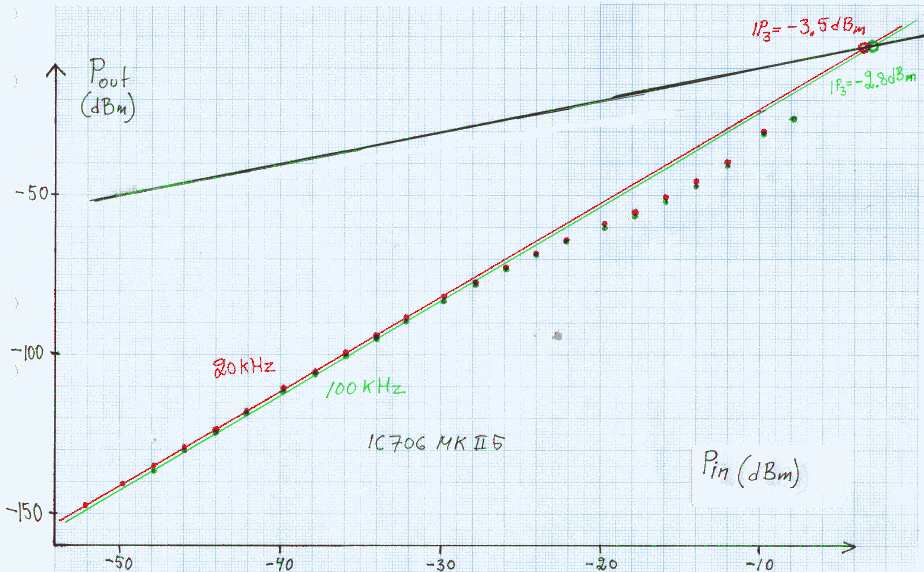
Fig.12. IM3 data for the IC706MKIIG. |
|
The IC706MKIIG is well characterized by the IP3 number which is about -3 dBm both at 20 kHz and at 100 kHz. When looking at the difference between the measured IM3 levels and the theoretical computed from 2 * P2 + P3, one finds an error of -8.5 dB at 20 kHz and an error of -7.5 dB at 20 kHz. The formula would be correct if IP3 were 0 dBm. The full formula is P1 - IP3= 2 * (P2 - IP3) + (P3 - IP3). This means that IP3 is half the errors, -4.2 dBm at 20 kHz and -3.8 dBm at 100 kHz. The values obtained graphically from an extrapolation in figure 12 are less accurate, but fairly close. Presumably the first IF filter is narrow enough to not allow both signals to pass in which case the IP3 number is IP3 for the front-end. The noise figure is 12.1 dB. The intermodulation level follows the third order law up to about -33 dBm where the deviation is about 0.5 dB. IM3 is then about 60 dB below the two tones. IM3 in FT1000DThe FT1000 has a front-end AGC. At at the point where it starts to reduce the signal, intermodulation generated in the mixer will be reduced. The minimum front-end intermodulation occurs when the RF volume is set for the S-meter to show S9+60 dB. The input signal required to reach this level is +8 dBm. At higher attenuation, the intermodulation caused by the attenuator diodes increases and dominates over the intermodulation in the mixer.The front end AGC uses a PIN(?)-diode attenuator and it has some effect on the input impedance of the FT1000 unit. Small changes on the input impedance are visible already at an S-meter reading of S9, corresponding to a signal level of -46 dBm or two equally strong signals at -52 dBm. With an IP3 in the order of +21 dBm, the FT1000 will have an IM3 level of -52 dBm for an input signal in the order of -3 dBm. With the "pilot tone" from generator (1) at -52 dBm present simultaneously, based on the observation that the impedance starts changing when the meter is at S9, the IM3 measurements can be expected to deviate from the third order law due to the AGC when IM3 is about 50 dB below the test signals. This means that the IP3 measurements should be unaffected by the front end AGC at levels where the third order law usually is accurate within 0.5 dB. Figure 13 shows the measured result for the FT1000D at 20 kHz and at 100 kHz. The frequency stability is very good when an external fan is used to prevent the built-in fan from going on and off so it is possible to follow the IM3 product deep down into the noise. The bandwidth was 0.5 Hz with an S-meter averaging time of 10 minutes for the lowest readings where the IM3 product was only about 6dB above the noise in 0.5 Hz bandwidth. The raw data ft1000_20.txt and ft1000_100.txt with the set-up of figure 11 and ft1000_20att.txt and ft1000_100att.txtwith a 20 dB attenuator added were processed with calim.f and the output from gencal.f (see above) to produce the data files ft1000a20.txt and ft1000a20att.txt for 20 kHz separation and ft1000a100.txt and ft1000a100att.txt for 100 kHz separation. There are several deviations from the third order law. First of all, adding a 20 dB attenuator forces the notch filter to work with 20 dB higher signal levels which will make the intermodulation caused by the quartz crystals to be 60 dB higher than without the attenuator. The attenuator will of course attenuate the intermodulation products by 20 dB but still the ratio signal to IM3 will be degraded by 20 dB. |

Fig.13. IM3 in a FT1000D. Red is at a frequency separation of 20 kHz while green is at 100 kHz. Circles are with the set-up of figure 11 while '+' are with a 20 dB attenuator added. |
|
It is quite clear from figure 13 that power levels of about -23 dBm with the attenuator included are perturbed by intermodulation external to the FT1000 when the frequency separationis 20 kHz. Near this point adding a 2dB attenuator to the 20 dB attenuator actually increased the IM3 product. IM3 from the notch filter goes down by 2 dB while IM3 from the FT1000 goes down by 6 dB. What happens to the summed IM3 depands on the exact amplitude and phase relations. It is clear from the red Ý+Ý marks on figure 13 that the IM3 level out from the notch filter is at about -85 dBm for 20 kHz frequency separation when the signal pair is at -2 dBm. The red circles show that the FT1000 intermodulation is at -50 dBm for -2 dBm input. With the IM3 produced in the notch filter about 45 dB below the IM3 produced in the FT1000 when measuring without the 20 dB attenuator one might think the measurement is accurate. The amplitude ratio corresponding to 45 dB is about 180. Since the phase relation between the two intermodulation sources is unknown, the error is +/- 179/180 in amplitude which converts to 0.05 dB. A small error, but having the IM3 from the signal source suppressed by 20 dB only as is often considered satisfactory means that the amplitude uncertainty is 10 % which gives an uncertainty of 20 % or +/- 0.8 dB in the IM3 level. At a frequency separation of 100 kHz there is much less intermodulation produced in the quartz crystals and the test signal is probably accurate over the entire range of figure 13 when the 20 dB attenuator is not used. At 20 kHz there is a significant increase in IM3 level at about -15 dBm. This is the level where the S-meter just reaches zero. It is not an artifact or a measurement error, there is a phenomenon inside the FT1000 that raises the IM3 level by about 2 dB. At this signal level the AGC can be switched off without any effect at all on signal levels except that one does not have to average out the small amplitude variations that comes from the AGC system. At higher signal levels where AGC is active, the signal levels are perfectly stable with 3 decimals, the amplitudes are kept constant with a feed-back loop, the AGC. When the feed-back is broken because the signals do not reach the AGC threshold, there is a noise voltage that modulates the receiver gain at random causing a level uncertainty of about 0.05 dB. Switching the AGC off removes this uncertainty. As can be seen in the data files, the gain of the FT1000 increases by about 0.5 dB when the signal pair is added at 20 kHz frequency separation. This increased gain is caused exclusively by the nearest signal which is spaced 20 kHz away. The other test signal 40 kHz away does not affect the receiver gain This phenomenon, that the gain increases when a strong signal is added at a frequency separation of 20 kHz is unaffected by the RF gain setting up to S-meter readings of about S7, close to the point where one can see input impedance changes due to the front end AGC. It is clear that the FT1000 deviates slightly from the third order law at a frequency separation of 20 kHz. The discrepancy between IP3 values extrapolated from S5 and from the noise floor in 500 Hz bandwidth (-126 dBm) is about 1 dB so for all practical purposes the FT1000 IM3 is well characterized by an IP3 value of +22 dBm. The noise figure is 19.3 dB To SM 5 BSZ Main Page |