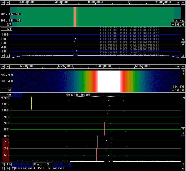
Fig 1.A strong signal received in a wide filter (7kHz) produced by back-transforming 57 out of the 512 bins of fft3 (9 in the upper right corner of of the spectrum gives the fft3 size as 29=512.) The window used is sin2
Theoretical background.When we sample a radio signal in e.g. 8192 sucessive digital values using an A/D converter and compute the spectrum by use of some computer code that implements an FFT algorithm, the spectrum obtained is NOT the spectrum of the signal we have sampled. It is the spectrum of an infinite series of the N samples repeated over and over again. The signal itself and its derivatives at point N-1 will generally not fit well to the signal at point 0 of the next repetition. The signal amplitude and curvature will change abruptly from one point to the next and that corresponds to a wideband pulse. Such pulses are artifacts and they destroy the dynamic range of the FFT as a spectral analysis tool.The way to solve this problem is to multiply the N samples with a window function such that all the values near points 0 and N-1 become very close to zero. This way the signal at 0 and N-1 will match each other very closely. The spectrum is of course no longer the spectrum of the signal present at the antenna, it is the antenna signal modulated by the window function. The Fourier transform is a linear process. It is enough to analyze its behaviour for a single signal to understand the behaviour in general. When no window is used the FFT output for a single sine wave depends very strongly on whether the signal goes even in the time interval spanned by the samples. In case the signal goes even exactly, there will be no discontinuity and then all the signal energy goes into a single FFT bin. On the other hand, if the signal goes X+0.5 periods in the time span, there will be a voltage jump of twice the signal amplitude from one point to the next or a corresponding jump in the derivatives. As an artefact the spectrum of such voltage spikes contribute to the spectrum. This link Sliding FFT and DSP filtering. discusses FFT and windowing in some detail. The Linrad baseband filterWhen the signal is frequency converted for the intertesting part to be centered around zero and down sampled to a sampling rate not much larger than needed for the frequency band of interest, the time function carrying the signal in Linrad is called timf3.Linrad computes an FFT labeled fft3, and the signals actually processed and sent to the loudspeaker are derived from a back transformation of fft3 in which frequency bins outside the range of interest are set to zero. When the number of bins used (not set to zero) is large, the exact response of each individual bin is not of much interest. Figure 1 shows a typical Linrad screen with a modest transform size, yet large enough to make the filter representation as a perfectly rectangular response reasonably valid. In figure 1, a signal at 10.6805 MHz received by a Perseus HF receiver. The level is 0.2 dB below A/D saturation. There is a second signal 100 dB below the main signal at about 10.694, but that is of no interest on this page. The signal is recorded data from the Hard disk. |
|
Fig 1.A strong signal received in a wide filter (7kHz) produced by back-transforming 57 out of the 512 bins of fft3 (9 in the upper right corner of of the spectrum gives the fft3 size as 29=512.) The window used is sin2 |
|
Figure 1 is produced with Linrad-03.00 so it takes bin response into account,
but the effect is if no significance here.
This figure is actually presented first on this page to show that not
much has been changed.
With normal settings for the spectrum Y scale, the contributions
from including the sin2 window is not noticeable
when as much as 50 bins are selected for the filter.
Figure 2 shows exactly the same thing. Here the vertical scale extends over the about 110 dB that is the dynamic range of the Perseus HF receiver at the bin bandwidth of fft3. It is pretty obvious that the passband edges have a shape that is related to the shape of the signal itself. Linrad-02.58 and earlier would have shown vertical lines down to the spectrum bottom right at the corners, what is new in 03.00 is that the true response is computed. When as few as 50 points are selected, what looks like a perfect rectangular filter in previous Linrad versions is actually a filter that only falls to about -85 dB for twice the bandwidth. Larger transforms with more bins for the same bandwidth improves the fiter shape factor, but there is a cost in processing delay. |

Fig 2. The same as figure 1 with but with an increased vertical scale range. |
The spectral shape for a single bin.Linrad computes the spectral response for an individual bin by computing the average power spectrum of a sinewave that sweeps over the frequency range of a single bin. From -0.5 to +0.5 times the frequency bin separation. This way all possible phases are averaged.Figure 3 shows the theoretical filter response for a single bin with the sin2 window and the Perseus signal. (The same as used in figures 1 and 2.) The theoretical spectrum is closely similar to the observed spectrum. It is possible to make the observed spectrum narrower by carefully tuning the signal to fit exactly on a bin. Figure 3 as well as all the figures below show the spectrum with the Perseus signal right between two bins. It is pretty clear that a filter like the one in figure 3 would be perfectly adequate for weak signal work when no strong signal is present close to the desired signal. Using only a single bin means that the time delay can be made extremely short. For a bandwidth of 250 Hz, the transform would only have to span 8 milliseconds. On crowded bands where a signal 90 dB above the one of interest is likely to occur a couple of kHz away, this filter would not be adequate. |
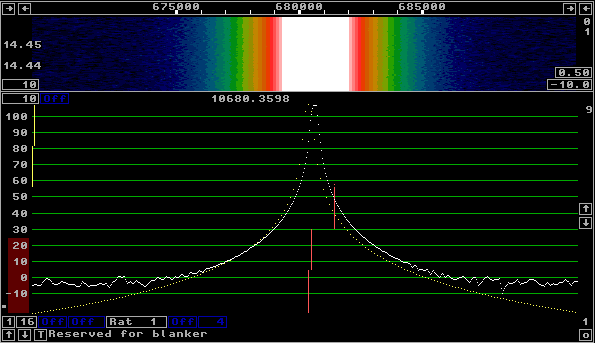
Fig 3. The bin response of the sin2 window. |
| Figure 4 shows the response of a sin1 window (the sine function itself.) It gives a significantly narrower bandwidth for the same time delay, but stop band rejection is worse compared to the sin2 window. |

Fig 4. The bin response of the sin 1 window. |
| Higher powers of sin give wider filters with steeper skirts. Figures 5 and 6 show sin3 and sin4 respectively. |
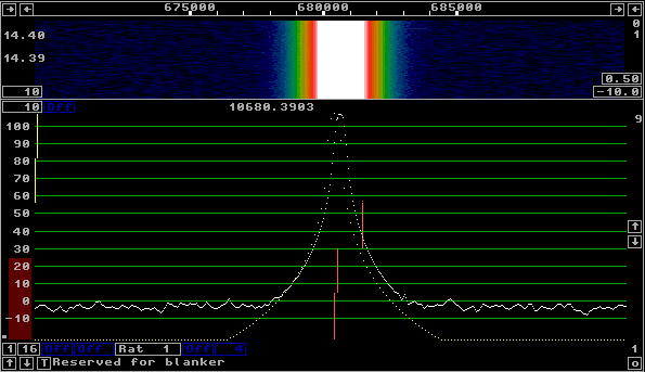
Fig 5. The bin response of the sin3 window. |

Fig 6. The bin response of the sin4 window. |
|
The Gaussian window which is shown in figure 7 should be the optimum
window in some sense since this curve form is the mathematical expression
that allows the narrowest possible peak in the time domain as well
as in the frequency domain simultaneously.
The FFT of a Gaussian is another Gaussian.
|
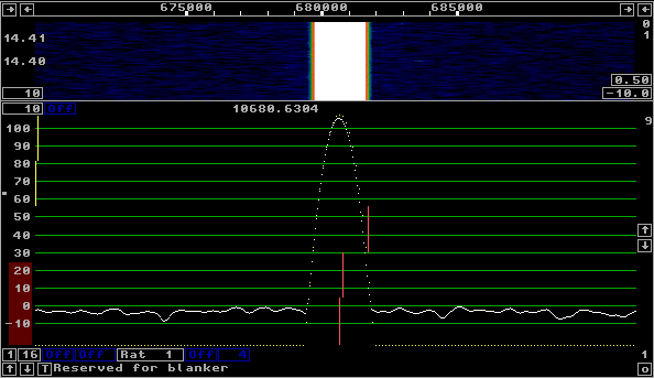
Fig 7. The bin response of the Gaussian window. |
|
The flat window with rise and fall curve forms generated by the Gaussian
error function erf(x) combines a very narrow bandwidth at e.g. -10 dB
with a rather slow fall-off at high attenuations. See figure 8.
The slow fall-off, about 10 times slower as compared to the Gaussian
is caused by the about 10 times faster fall-off in the window function
while the narrow bandwidth is generated by the long flat center part
of the window function.
|
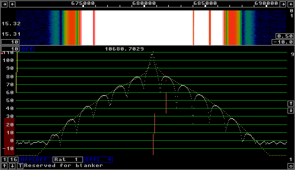
Fig 8. The bin response of the flat window with erf(x) fall-off. |
|
The selection of an optimum window function is important only
when very fast response is desired through the use of
small fft3 transforms.
It should be easy to decide how steep skirts one might need
in a particular situation since the baseband spectrum displays
the signals actually present in the same scale as it shows the
frequency response of the baseband filter with yellow dots.
To SM 5 BSZ Main Page |